Compilation of Examples
In this document, we present the compilation of 10 relational differentially private queries into the corresponding SQL queries, targeting SQLite and PostgreSQL.
1. Query Language
As ways of presenting the examples, we use the notation of DPella queries. DPella is a domain-specific language for writing differentially private queries. It is designed to be expressive and user-friendly, allowing users to write DP-queries in a procedural style. While this report uses DPella as the reference language, the concepts and techniques presented can be adapted to other languages or frameworks that support the same differential private primitives.
1.1. Basic Definitions
-
Types: The query language supports the following basic types:
- $\mathbb{B} = {\text{true}, \text{false}}$ (boolean)
- $\mathbb{Z}$ (integer)
- $\mathbb{R}$ (double)
- $\text{String}$ (text)
- Row: A row $r$ is a finite mapping from column names to values:
- $r: \text{ColName} \rightarrow V$
- $V = \mathbb{B} \cup \mathbb{Z} \cup \mathbb{R} \cup \text{String} \cup E$ (value universe)
- $\text{ColName}$ (column names): A finite set of string identifiersXS
- $\text{dom}(r)$ denotes the set of column names defined in $r$
-
Table: A table $T$ is an ordered sequence of rows with a consistent schema:
- $T = \langle r_1, r_2, \ldots, r_n \rangle$ where each $r_i \in \text{Row}$
- All rows in $T$ have the same domain: $\forall r_i, r_j \in T: \text{dom}(r_i) = \text{dom}(r_j)$
- $\text{schema}(T) = \text{dom}(r_i)$ for any $r_i \in T$ (the set of column names)
1.2. Core Operations
We classify the core operations of the query language into two categories: Transformations and Measurements:
- Transformations: These operations modify the structure or content of tables without changing their fundamental nature. In other words, transformations are use to manipulate the data and prepare it for analysis. The following transformations are supported:
- Projection: Selects specific columns from a table
- Selection/Filtering: Filters rows based on a condition
- Creation: Create a new column
- Classification: Classify rows into a categorical value based on a condition
To express predicates and intermediate results, the language supports the following operations:
- Comparison: $<, \leq, >, \geq, =, \neq$
- Arithmetic: $+, -, \times, \div, \bmod$
- Boolean: $\land$ (AND), $\lor$ (OR), $\neg$ (NOT)
- Measurements: These operations compute statistics or aggregations over the data, while preserving differential privacy. Measurements are used to extract insights from the data while ensuring that individual contributions remain private. The following measurements are supported:
- Count: Counts the number of rows in a table
- Sum: Computes the sum of a numeric column
- Partition: A special kind of measurement that returns multiple results. This operation groups rows by a the unique values of a specified set of columns and applies a measurement to each group, returning a table with the results. This operation is similar to the SQL
GROUP BYclause, however, it restricts the operations that can be applied to the grouped data to exactly one measurement, which can be eitherCountorSum.
1.3. Query Structure
A query is a composition of zero or more transformations followed by exactly one measurement. The structure of a query can be represented as follows:
query_body ::= (transformation;)* measurement
where transformation and measurement refer to the operations listed above, and ; denotes the sequence operator. The language supports query naming via the let <query_name> = {<query_body>} construct, allowing users to define reusable queries.
To execute a query on a table, we use the notation execute <query_name>(<table_name>) with budget (epsilon <budget_value>), where <table_name> is the name of the table to be queried. The result of the query is a table containing the computed statistics or aggregations.
2. Query Compilation
The compilation process involves translating the DPella queries into SQL queries that can be executed on a relational database. The compilation is done in a way that preserves the differential privacy guarantees of the original DPella queries. The compilation process includes the following steps:
- Mapping Transformations to SQL: Each transformation is mapped to the corresponding SQL operation. This includes translating projections, selections, and classifications into SQL
SELECT,WHERE, andCASEstatements, respectively. - Mapping Measurements to SQL: The measurements are translated into SQL aggregate functions, such as
COUNTandSUM. - Handling Differential Privacy:
The compiled SQL queries are enhanced with mechanisms to guarantee differential privacy, typically by adding noise to measurement results. As detailed in our previous reports (see interoperability-report and technical-report), we describe how to integrate custom noise-generating functions into various SQL engines. Specifically, we introduce the
dpella_sample_randomfunction, which takes as arguments the true value to be perturbed and the scale parameter for the Laplace mechanism. This function can be incorporated directly into SQL queries to ensure differential privacy. For instance, a measurement such asSUM(<column>)can be rewritten asdpella_sample_random(SUM(<column>), <scale>), where<scale>is calculated during compilation as $\frac{\Delta_f}{\varepsilon}$, with $\Delta_f$ representing the sensitivity of the aggregation function. To ensure the true value has the expected type, we cast the aggregation result toREALbefore applying the noise function, as demonstrated in the SQL examples below. - Generating the Final SQL Query: The final SQL query is generated by combining the transformed operations and measurements, ensuring that the query adheres to the syntax and semantics of the target SQL dialect (e.g., SQLite or PostgreSQL).
Key idea: The body of the query is a sequence of transformations followed by a measurement. This can be represented as a WITH clause in SQL, where each transformation is represented as a subquery. The final measurement is then applied to the result of the last transformation. This approach mirrors the procedural structure of the original query and enables modular, readable, and efficient SQL generation.
When compiling a query, we start with the original table, which we refer to as main_0 (where the subscript indicates the step in the transformation sequence) or <query_name>_0 to improve readability. For each transformation in the query, we introduce a new subquery, incrementing the index each time: main_1, main_2, and so on. Each subquery operates on the result of the previous one, so main_{i+1} is defined in terms of main_{i}. This systematic naming and chaining of subqueries within the WITH clause allows us to clearly represent the sequence of transformations. The final measurement is then applied to the last subquery, main_n, where n is the total number of transformations. This approach provides a modular and traceable structure for the compiled SQL, making it easy to follow the flow from the original table through each transformation to the final result.
2.2. SQL constructs
Now that we have a general understanding of the query language and the compilation strategy, we can delve into the specific SQL constructs used to implement the transformations and measurements. For each operation we provide DPella syntax, followed by the corresponding SQL sub-query syntax. The SQL queries are designed to be compatible with both SQLite and PostgreSQL, ensuring that the compiled queries can be executed in either database system. Later on, we’ll discuss the specific differences between the two SQL dialects, if any, and how they affect the compilation process.
- Transformations:
- Projection:
project (c_1, c_2, ..., c_n)main_<idx+1> AS ( SELECT c_1, c_2, ..., c_n FROM main_<idx> )- Selection/Filtering:
filter <condition>
main_<idx+1> AS ( SELECT * FROM main_<idx> WHERE <condition> )- Creation
let <new_column> = <expr>main_<idx+1> AS ( SELECT *, <expr> AS <new_column> FROM main_<idx> ) - Classification
 let <new_column> = classify {
case <condition_1> : <value_1>
case <condition_2> : <value_2>
...
case <condition_n> : <value_n>
default: <default_value>
 }
main_<idx+1> AS ( SELECT *, CASE WHEN <condition_1> THEN <value_1> WHEN <condition_2> THEN <value_2> ... WHEN <condition_n> THEN <value_n> ELSE <default_value> END AS <new_column> FROM main_<idx> ) -
Measurements:
- Count:
count
main_<idx+1> AS ( SELECT dpella_sample_random(CAST (COUNT(*) AS REAL), <scale>) AS dp_count FROM main_<idx> )- Sum:
sum(<column>)main_<idx+1> AS ( SELECT dpella_sample_random(CAST (SUM(<column>) AS REAL), <scale>) AS dp_sum FROM main_<idx> ) - Partition:
```
partition (
, , ...) repeat { }
 In it's simplest form, the partition operation can be expressed as:
 ```sql
   main_<idx+1> AS (
     SELECT
       <column_1>,
       <column_2>,
       ...,
       dpella_sample_random(CAST (<measurement> AS REAL), <scale>) AS dp_<measurement>
     FROM main_<idx>
     GROUP BY <column_1>, <column_2>, ...
   )
However, we opt for a more controlled representation that i) ensures that the number of groups is not unbounded, and ii) prepares the compilation for more expressive partition queries that allows sub-queries (not just measurements) as the computation to be performed on the partitions. In this case, we use a
VALUESclause to define the unique values of the partition columns, and then join it with the main table to compute the measurement for each group:-- create a table containing the known values of the key column1 <column1_enum> (x) AS ( VALUES (<value_1>) UNION ALL VALUES (<value_2>) ... UNION ALL VALUES (<value_n>) ), -- create a table containing the known values of the key column2 <column2_enum> (x) AS ( VALUES (<value_1>) UNION ALL VALUES (<value_2>) ... UNION ALL VALUES (<value_m>) ), ..., main_<idx+1> AS ( SELECT <column1_enum>.x, <columl2_enum>.x, ..., dpella_sample_random( -- the measurement is computed as a subquery that aggregates the main table based on the values of the -- partition columns. This will allow for more transformations to be defined within the query that is -- applied to each partition -- -- We use COALESCE to ensure that if the measurement is NULL (e.g., no rows match the conditions), -- the "real value" is set to 0.0 instead, and we avoid reveling the absence of data. SELECT COALESCE(CAST (<measurement> AS REAL), 0.0) FROM main_<idx> -- the following WHERE clause ensures that we only consider rows that match the current group of interest -- defined by the values of the partition columns WHERE (<column1_enum>.x = main_<idx>.<column_1>) AND (<column2_enum>.x = main_<idx>.<column_2>) AND ... , <scale>) FROM <column1_enum>, <column2_enum>, ... GROUP BY <column1_enum>.x, <column2_enum>.x, ... ) - Count:
3. Example Queries
In this section, we present 10 example queries using the features of the query language described above. Each query is designed to demonstrate different aspects of the language, including transformations, measurements typically used for data analysis, and the application of differential privacy.
All the examples are designed to be executed on a table named employees, which containing information about a hospital’s staff. The schema of the employees table is as follows:
full_name: Name of the employee (string)age: Age of the employee (integer)job: Employee’s job title, either “doctor”, “nurse” or “manager” (enumeration)part-time: Whether the employee works part-time (boolean)worked_hours: Number of hours worked by the employee (double)accumulated_holidays: Number of accumulated holidays (integer)
Query 1: Simple Measurement
Count the total number of employees:
let q1 = {
  count
}
Query 2: Project and Sum
Calculate the total accumulated holidays for all employees:
let q2 = {
  project accumulated_holidays;
  sum
}
Query 3: Filter, Project, and Sum
Calculate the total accumulated holidays for part-time employees:
let q3 = {
  filter part_time;
  project accumulated_holidays;
  sum
}
Query 4: Complex Filter with Boolean Operations
Count doctors who work part-time or work more than 40 hours:
let q4 = {
  filter job == job.doctor && (part_time || worked_hours > 40.0);
  count
}
Query 5: Sequential filters
Count young employees (age < 30) who are part-time nurses and have accumulated more than 10 holidays:
let q5 = {
  filter age < 30;
  filter job == job.nurse;
  filter part_time;
  filter accumulated_holidays > 10;
  count
}
Query 6: Create Column with Arithmetic
Calculate employees’s remaining holidays after a mandatory break of 5 days, then count the number of employees with holidays after break greater than 10:
let q6 = {
  create holidays_after_break = accumulated_holidays - 5;
  filter holidays_after_break > 10;
  count
}
Query 7: Classify Operation
Categorize employees into “senior” if age > 50, “adult” if age in (30, 50], and “junior” otherwise, then count the number of senior nurses:
let q7 = {
  create age_class = classify {
    case age > 50 : senior
    case age > 30 : adult
    default : junior
  };
  filter job == job.nurse && age_class == age_class.senior;
  count
}
Query 8: Partition Operation
Count the number of employees that are working part-time and those that are full-time:
let q8 = {
  partition part_time repeat {
    count
  }
}
Query 9: Cross-tabulation with partition
Sum the accumulated holidays of the employees classified by seniority and part-time status:
let q9 = {
  create is_senior = age > 50;
  partition (is_senior, part_time) repeat {
    sum(accumulated_holidays);
  }
}
Query 10: Several operation in a single query
Calculate the total holidays of senior that are not doctors and have worked more than 30 hours using multiple-column projection and sequential filters
let q10 = {
  project (age, job, worked_hours, accumulated_holidays);
  filter job != job.doctor && worked_hours > 30.0;
  create age_class = classify {
    case age > 50 : senior
    case age > 30 : adult
    default : junior
  };
  filter age_class == age_class.senior;
  sum(accumulated_holidays);
}
3.1. Compilation into optimized SQLite queries
Query 1: Simple Measurement
WITH
  q1_0 (full_name, age, job, part_time, worked_hours, accumulated_holidays) AS (
    SELECT * FROM DPELLA_EMPLOYEES),
  q1_1 (dp_count) AS (
    SELECT dpella_sample_random(CAST (COUNT(*) AS REAL), 10.0) FROM q1_0)
SELECT q1_1.dp_count FROM q1_1
Query 2: Project and Sum
WITH
  q2_0 (full_name, age, job, part_time, worked_hours, accumulated_holidays) AS (
    SELECT * FROM DPELLA_EMPLOYEES),
  q2_1 (dp_sum) AS (
    SELECT dpella_sample_random(CAST (SUM(q2_0.accumulated_holidays) AS REAL), 400.0)
    FROM q2_0)
SELECT q2_1.dp_sum FROM q2_1
Optimization #1: Queries using the combination project <column_name>; sum can be optimized by directly applying the SUM operation over the numeric column, SELECT SUM(<column_name>), instead of projecting the column first. This reduces the number of intermediate subqueries to be produced, making the SQL compilation more readable.
Query 3: Filter, Project, and Sum
WITH
  q3_0 (full_name, age, job, part_time, worked_hours, accumulated_holidays) AS (
    SELECT * FROM DPELLA_EMPLOYEES),
  q3_1 (dp_sum) AS (
    SELECT dpella_sample_random(CAST (SUM(q3_2.accumulated_holidays) AS REAL), 400.0)
    FROM q3_0
    WHERE q3_0.part_time)
SELECT q3_1.dp_sum FROM q3_1
Optimization #2: Queries using the combination filter <condition>; <measurement> can be optimized to directly apply the measurement over the filtered rows, i.e., SELECT <measurement> FROM <table> WHERE <condition>, instead of creating an intermediate subquery to filter the rows, followed by another subquery to apply the measurement.
Observe that the optimizations are compounded, this query uses the project <column_name>; sum optimization, and the filter <condition>; <measurement> optimization, resulting in a single subquery that applies the measurement directly over the filtered rows.
Query 4: Complex Filter with Boolean Operations
WITH
  q4_0 (full_name, age, job, part_time, worked_hours, accumulated_holidays) AS (
    SELECT * FROM DPELLA_EMPLOYEES),
  q4_1 (dp_count) AS (
    SELECT dpella_sample_random(CAST (COUNT(*) AS REAL), 10.0)
    FROM q4_0
    WHERE (q4_0.job = 0) AND (q4_0.part_time OR (q4_0.worked_hours > 40.0)))
SELECT q4_1.dp_count FROM q4_1
Note: This query uses the filter <condition>; <measurement> optimization, where the condition is a complex boolean expression combining multiple conditions with logical operators, and the measurement is a count of the rows that satisfy the condition.
Query 5: Sequential filters
WITH
  q5_0 (full_name, age, job, part_time, worked_hours, accumulated_holidays) AS (
    SELECT * FROM DPELLA_EMPLOYEES),
  q5_1 (dp_count) AS (
    SELECT dpella_sample_puredp_laplace(CAST (COUNT(*) AS REAL), 10.0)
    FROM q5_0
    WHERE (q5_0.accumulated_holidays > 10) AND (q5_0.part_time) AND (q5_0.job = 1) AND (q5_0.age < 30))
SELECT q5_1.dp_count FROM q5_1
Optimization #3: Queries sequencing different filters filter <condition_1>; filter <condition_2>; ... ; filter <condition_n>; ... can be optimized to a single subquery that applies all the filters in a single WHERE clause, with the AND operator combining the conditions, i.e., SELECT ... FROM <table> WHERE <condition_1> AND <condition_2> AND ... AND <condition_n>.
Query 6: Create Column with Arithmetic
WITH
  q6_0 (full_name, age, job, part_time, worked_hours, accumulated_holidays) AS (
    SELECT * FROM DPELLA_EMPLOYEES),
  q6_1 (dp_count) AS (
    SELECT dpella_sample_random(CAST (COUNT(*) AS REAL), 10.0)
    FROM q6_0
    WHERE ((q6_0.accumulated_holidays - 5) > 10))
SELECT q6_1.dp_count FROM q6_1
Optimization #4: Queries using the combination create <new_column> = <expr>; filter <condition_new_column>; ... can be optimized to a single subquery that applies the arithmetic expression in the filter expression instead of creating a new column that is later filtered. This can be expressed as
SELECT ... FROM <table> WHERE <condition_over_expr>. This optimization should not be applied if the new column is used in subsequent transformations or measurements, as it would require the column to be created first.
Query 7: Classify Operation
WITH
  q7_0 (full_name, age, job, part_time, worked_hours, accumulated_holidays) AS (
    SELECT * FROM DPELLA_EMPLOYEES),
  q7_1 (dp_count) AS (
    SELECT dpella_sample_random(CAST (COUNT(*) AS REAL), 10.0)
    FROM q7_0
    WHERE
      (q7_0.job = 1) AND
      ((CASE WHEN (q7_0.age > 50) THEN 0
             WHEN (q7_0.age > 30) THEN 1
             ELSE 2 END) = 0))
SELECT q7_1.dp_count FROM q7_1
Note: This query uses the create <new_column> = <expr>; filter <condition_new_column>; ... optimization, where the expression is a classification operation translating to a CASE WHEN statement in SQLite.
Query 8: Partition Operation
WITH
  q8_0 (full_name, age, job, part_time, worked_hours, accumulated_holidays) AS (
    SELECT * FROM DPELLA_EMPLOYEES),
  part_time_enum (x) AS (
    VALUES (FALSE)
      UNION ALL
    VALUES (TRUE)),
  q8_1 (part_time, dp_count) AS (
    SELECT
      part_time_enum.x,
      dpella_sample_random(
        (SELECT COALESCE(CAST (COUNT(*) AS REAL), 0.0)
         FROM q8_0
         WHERE (q8_0.part_time = part_time_enum.x)),
        10.0)
    FROM part_time_enum
    GROUP BY part_time_enum.x)
SELECT q8_1.part_time, q8_1.dp_count FROM q8_1
Query 9: Cross-tabulation with partition
WITH
  q9_0 (full_name, age, job, part_time, worked_hours, accumulated_holidays) AS (
    SELECT * FROM DPELLA_EMPLOYEES),
  q9_1 (full_name, age, job, part_time, worked_hours, accumulated_holidays, is_senior) AS (
    SELECT
      q9_0.full_name,
      q9_0.age,
      q9_0.job,
      q9_0.part_time,
      q9_0.worked_hours,
      q9_0.accumulated_holidays,
      (q9_0.age > 50) AS is_senior
    FROM q9_0),
  is_senior_enum (x) AS (
    VALUES (FALSE)
    UNION ALL
    VALUES (TRUE)),
  part_time_enum (x) AS (
    VALUES (FALSE)
    UNION ALL
    VALUES (TRUE)),
  q9_2 (is_senior, part_time, dp_sum) AS (
    SELECT
      is_senior_enum.x,
      part_time_enum.x,
      dpella_sample_random(
        (SELECT COALESCE(CAST (SUM(q9_1.accumulated_holidays) AS REAL), 0.0)
         FROM q9_1
         WHERE ((q9_1.is_senior = is_senior_enum.x) AND (q9_1.part_time = part_time_enum.x))),
        400.0)
    FROM is_senior_enum, part_time_enum
    GROUP BY is_senior_enum.x, part_time_enum.x)
SELECT q9_2.is_senior, q9_2.part_time, q9_2.dp_sum FROM q9_2
Note: Different from previous queries where the definition of a new column was not reflected as a new subquery in the WITH clause, this query generates the q9_1 table creating the is_senior column, which is then used in the partition operation. We don’t “optimize” away the creation of the is_senior column, as i) it is relevant for the subquery generating the possible values and ii) it is used in the partition operation, which requires the column to be defined first in order to filter the correct group of rows (e.g., WHERE ((q9_1.is_senior = is_senior_enum.x) AND (q9_1.part_time = part_time_enum.x))).
Query 10: Several operation in a single query
WITH
  q10_0 (full_name, age, job, part_time, worked_hours, accumulated_holidays) AS (
    SELECT * FROM DPELLA_EMPLOYEES),
  q10_1 (dp_sum) AS (
    SELECT dpella_sample_random(CAST (SUM(q10_0.accumulated_holidays) AS REAL), 400.0)
    FROM q10_0
    WHERE
      ((CASE WHEN (q10_0.age > 50) THEN 0
             WHEN (q10_0.age > 30) THEN 1
             ELSE 2 END) = 0) AND
      (q10_0.job != 0) AND
      (q10_0.worked_hours > 30.0))
SELECT q10_1.dp_sum FROM q10_1
Optimization #5: Queries using projections that do not affect the final measurement can be optimized to remove the projection step, i.e., project <column_name>; <measurement> can be optimized to SELECT <measurement> FROM <table>. In this case, the project (age, job, worked_hours, accumulated_holidays) step is not necessary for the final measurement, which is a sum of the accumulated_holidays column. Therefore, we can directly apply the SUM operation over the accumulated_holidays column in the SELECT statement.
3.2. Compilation into optimized PostgreSQL queries
Query 1: Simple Measurement
WITH
  q1_0 (full_name, age, job, part_time, worked_hours, accumulated_holidays) AS (
    SELECT * FROM DPELLA_EMPLOYEES),
  q1_1 (dp_count) AS (
    SELECT dpella_sample_random(CAST (COUNT(*) AS FLOAT8), 10.0) FROM q1_0)
SELECT q1_1.dp_count FROM q1_1
Query 2: Project and Sum
WITH
  q2_0 (full_name, age, job, part_time, worked_hours, accumulated_holidays) AS (
    SELECT * FROM DPELLA_EMPLOYEES),
  q2_1 (dp_sum) AS (
    SELECT dpella_sample_random(CAST (SUM(q2_0.accumulated_holidays) AS FLOAT8), 400.0)
    FROM q2_0)
SELECT q2_1.dp_sum FROM q2_1
Query 3: Filter, Project, and Sum
WITH
  q3_0 (full_name, age, job, part_time, worked_hours, accumulated_holidays) AS (
    SELECT * FROM DPELLA_EMPLOYEES),
  q3_1 (dp_sum) AS (
    SELECT dpella_sample_random(CAST (SUM(q3_2.accumulated_holidays) AS FLOAT8), 400.0)
    FROM q3_0
    WHERE q3_0.part_time)
SELECT q3_1.dp_sum FROM q3_1
Query 4: Complex Filter with Boolean Operations
WITH
  q4_0 (full_name, age, job, part_time, worked_hours, accumulated_holidays) AS (
    SELECT * FROM DPELLA_EMPLOYEES),
  q4_1 (dp_count) AS (
    SELECT dpella_sample_random(CAST (COUNT(*) AS FLOAT8), 10.0)
    FROM q4_0
    WHERE (q4_0.job = 0) AND (q4_0.part_time OR (q4_0.worked_hours > 40.0)))
SELECT q4_1.dp_count FROM q4_1
Query 5: Sequential filters
WITH
  q5_0 (full_name, age, job, part_time, worked_hours, accumulated_holidays) AS (
    SELECT * FROM DPELLA_EMPLOYEES),
  q5_1 (dp_count) AS (
    SELECT dpella_sample_puredp_laplace(CAST (COUNT(*) AS FLOAT8), 10.0)
    FROM q5_0
    WHERE (q5_0.accumulated_holidays > 10) AND (q5_0.part_time) AND (q5_0.job = 1) AND (q5_0.age < 30))
SELECT q5_1.dp_count FROM q5_1
Query 6: Create Column with Arithmetic
WITH
  q6_0 (full_name, age, job, part_time, worked_hours, accumulated_holidays) AS (
    SELECT * FROM DPELLA_EMPLOYEES),
  q6_1 (dp_count) AS (
    SELECT dpella_sample_random(CAST (COUNT(*) AS FLOAT8), 10.0)
    FROM q6_0
    WHERE ((q6_0.accumulated_holidays - 5) > 10))
SELECT q6_1.dp_count FROM q6_1
Query 7: Classify Operation
WITH
  q7_0 (full_name, age, job, part_time, worked_hours, accumulated_holidays) AS (
    SELECT * FROM DPELLA_EMPLOYEES),
  q7_1 (dp_count) AS (
    SELECT dpella_sample_random(CAST (COUNT(*) AS FLOAT8), 10.0)
    FROM q7_0
    WHERE
      (q7_0.job = 1) AND
      ((CASE WHEN (q7_0.age > 50) THEN 0
             WHEN (q7_0.age > 30) THEN 1
             ELSE 2 END) = 0))
SELECT q7_1.dp_count FROM q7_1
Query 8: Partition Operation
WITH
  q8_0 (full_name, age, job, part_time, worked_hours, accumulated_holidays) AS (
    SELECT * FROM DPELLA_EMPLOYEES),
  part_time_enum (x) AS (
    VALUES (FALSE)
      UNION ALL
    VALUES (TRUE)),
  q8_1 (part_time, dp_count) AS (
    SELECT
      part_time_enum.x,
      dpella_sample_random(
        (SELECT COALESCE(CAST (COUNT(*) AS FLOAT8), 0.0)
         FROM q8_0
         WHERE (q8_0.part_time = part_time_enum.x)),
        10.0)
    FROM part_time_enum
    GROUP BY part_time_enum.x)
SELECT q8_1.part_time, q8_1.dp_count FROM q8_1
Query 9: Cross-tabulation with partition
WITH
  q9_0 (full_name, age, job, part_time, worked_hours, accumulated_holidays) AS (
    SELECT * FROM DPELLA_EMPLOYEES),
  q9_1 (full_name, age, job, part_time, worked_hours, accumulated_holidays, is_senior) AS (
    SELECT
      q9_0.full_name,
      q9_0.age,
      q9_0.job,
      q9_0.part_time,
      q9_0.worked_hours,
      q9_0.accumulated_holidays,
      (q9_0.age > 50) AS is_senior
    FROM q9_0),
  is_senior_enum (x) AS (
    VALUES (FALSE)
    UNION ALL
    VALUES (TRUE)),
  part_time_enum (x) AS (
    VALUES (FALSE)
    UNION ALL
    VALUES (TRUE)),
  q9_2 (is_senior, part_time, dp_sum) AS (
    SELECT
      is_senior_enum.x,
      part_time_enum.x,
      dpella_sample_random(
        (SELECT COALESCE(CAST (SUM(q9_1.accumulated_holidays) AS FLOAT8), 0.0)
         FROM q9_1
         WHERE ((q9_1.is_senior = is_senior_enum.x) AND (q9_1.part_time = part_time_enum.x))),
        400.0)
    FROM is_senior_enum, part_time_enum
    GROUP BY is_senior_enum.x, part_time_enum.x)
SELECT q9_2.is_senior, q9_2.part_time, q9_2.dp_sum FROM q9_2
Query 10: Several operation in a single query
WITH
  q10_0 (full_name, age, job, part_time, worked_hours, accumulated_holidays) AS (
    SELECT * FROM DPELLA_EMPLOYEES),
  q10_1 (dp_sum) AS (
    SELECT dpella_sample_random(CAST (SUM(q10_0.accumulated_holidays) AS FLOAT8), 400.0)
    FROM q10_0
    WHERE
      ((CASE WHEN (q10_0.age > 50) THEN 0
             WHEN (q10_0.age > 30) THEN 1
             ELSE 2 END) = 0) AND
      (q10_0.job != 0) AND
      (q10_0.worked_hours > 30.0))
SELECT q10_1.dp_sum FROM q10_1
3.3. Discussion
The examples above demonstrate the feasibility of compiling DP-queries into database-specific SQL queries that can be executed and verified against a reference implementation (see the next section for details on the testing methodology). Following are some relevant observations:
-
The initial sub-query (
<query_name>_0) that selects from the internal tableDPELLA_EMPLOYEESis not a necessary step if, at the moment of compilation, the table name is known. However, that is not the case for the DPella language, as the internal table names are not visible to the user. As such, the compilation process should be adapted to the specific access model for table-referencing in the target SQL dialect. -
Although using qualified names (e.g.,
q1_0.full_name) can make the generated SQL code more verbose, this approach is essential to maintain clarity and correctness, especially when targeting multiple SQL dialects. Qualified names prevent ambiguity in queries that involve several transformations or aggregations, where column names might otherwise overlap or be reused across subqueries. Additionally, they are valuable for debugging during compiler development, as they make it easier to trace errors back to their origin in the generated SQL. -
As is evident, targeting different SQL dialects requires minor adjustments to the generated SQL syntax — such as using
FLOAT8instead ofREALin PostgreSQL. In our process, we have found minimal differences, most of them are related to types and function names (e.g.,min/maxvs.least/greatest). These differences are manageable and do not significantly complicate the compilation process. Importantly, if the DP-language supports timestamps, they require special handling in the compilation process, as SQLite does not have a native timestamp type, while PostgreSQL does. In SQLite, timestamps are typically represented as integers (e.g., Unix timestamps), while in PostgreSQL, they can be represented asTIMESTAMPorTIMESTAMPTZtypes which we can take advantage of for better performance. This difference requires careful consideration during the compilation to ensure that the correct type is used in the generated SQL queries. -
Given the similarities between SQL dialects, we recommend compiling DP-queries to an intermediate representation: a dedicated SQL Abstract Syntax Tree (AST). This intermediate form can then be pretty-printed or rendered for the target database engine. By adopting this approach, the core compilation logic remains unified and maintainable, while only the final rendering step needs to account for dialect-specific differences. This avoids duplication of compilation code and streamlines support for multiple SQL backends.
-
Optimizing the generated SQL queries is essential for both readability and effective debugging. The optimizations described above — such as merging filters and measurements, and eliminating unnecessary projections — greatly improve the clarity and maintainability of the resulting SQL code. To systematically achieve these improvements, we recommend a two-phase compilation process: first, compile DP-queries into an intermediate representation (such as the previously mentioned SQL AST); then, apply optimizations to this intermediate representation before generating the final SQL code. This separation of concerns enables a more organized and maintainable compilation workflow, allowing optimizations to be applied in a structured manner without complicating the core compilation logic.
4. Testing Methodology
4.1. Differential Testing of DPella Implementations
Differential testing is a software testing technique where the same inputs are provided to multiple implementations of a system, and their outputs are compared to detect discrepancies. For DPella, this approach is particularly valuable as it allows us to verify the correctness of database-specific implementations against a reference implementation.
4.2. Overview
In the context of DPella, differential testing involves:
-
Reference Implementation: A native backend implementation that serves as the ground truth for query execution. This implementation directly interprets the formal semantics defined above and applies the differential privacy mechanisms as specified.
-
Database Backends: Implementations that translate DPella queries into database-specific SQL operations, using a zero-noise function for noise injection, meaning that no noise is added to results. This allows us to compare across implementations without having to account for statistical deviations.
-
Test Harness: Infrastructure that executes the same query across all backends and compares the results, checking that they produce exactly the same outputs.
-
Test Harness: Infrastructure that executes the same query across all backends and compares the results, checking that they produce exactly the same outputs.
In our case we will do the following:
- Execute the above queries using the native reference backend implementation.
- Execute the above queries using the SQLite backend implementation.
- Execute the above queries using the Postgres backend implementation.
- Compare the output of all, and ensure that there are no deviations between the three.
4.3. Results
We run the queries both using the native (core) engine, the SQLite engine, and the Postgres engine, and save the output. Note that we must take care to reset the engine between every experiment.
$ ./reset-engine.sh
$ dpella-repl -u root -p root -f ngi_examples.dpella --default-noise-source zero --stdin --engine=core > core-output
$ ./reset-engine.sh
$ dpella-repl -u root -p root -f ngi_examples.dpella --default-noise-source zero --stdin --engine=sqlite > sqlite-output
$ ./reset-engine.sh
$ dpella-repl -u root -p root -f ngi_examples.dpella --default-noise-source zero --stdin --engine="postgres://dpella:dpella@localhost:5432/dpella" > postgres-output
The contents of core-outuput will be the following:
dp_count
========
500.0


dp_sum
======
10518.0


dp_sum
======
5386.0


dp_count
========
153.0


dp_count
========
5.0


dp_count
========
319.0


dp_count
========
104.0


part_time  dp_count
=========  ========
false      256.0
true       244.0


is_senior  part_time  dp_sum
=========  =========  ======
false      false      2227.0
false      true       2150.0
true       false      2905.0
true       true       3236.0


dp_sum
======
3427.0
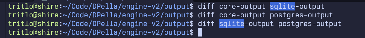
Now, we compare the three and ensure that they are all the same
  $ diff core-output sqlite-output
  $ diff core-output postgres-output
  $ diff sqlite-output postgres-output
As we get no output from any of the diff commands, this means that the output of all three is exactly the same, as expected.